/ʤiː-ʤiːkrəʊˈmætɪk/
![]()
![]()
![]()
The ‘ggchromatic’ package provides additional colour and fill scales to use with ‘ggplot2’ It uses the ‘ggplot2’ extension system to map a number of variables to different colour spaces with the ‘farver’ package. The package introduces ‘chromatic scales’, a term mirroring music terms. In music, chromatic scales cover all 12 notes. In ggchromatic, a chromatic scale can cover all channels in colour space. Admittedly, colour spaces might not be the most intuitive tool for interpreting a data visualisation, but can be useful for visualising less strict data impressions.
Installation
You can install the development of ggchromatic version from GitHub with:
# install.packages("devtools")
devtools::install_github("teunbrand/ggchromatic")
Example
These is a basic example of mapping three variables to the RGB colour space. This happens automatically for colours constructed by rgb_spec().
library(ggchromatic)
#> Loading required package: ggplot2

ggplot(mtcars, aes(mpg, disp)) +
  geom_point(aes(colour = cmy_spec(mpg, drat, wt)))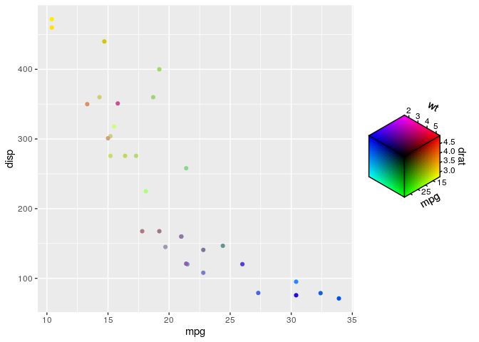
The associated scale functions give more options for customisation, like the HSV scale below.
df <- data.frame(
  x = c(row(volcano)), y = c(col(volcano)), z = c(volcano)
)

ggplot(df, aes(x, y, fill = hsv_spec(z, x, y))) +
  geom_raster() +
  scale_fill_hsv(limits = list(h = c(NA, 170)),
                 oob = scales::oob_squish,
                 channel_limits = list(h = c(0, 0.8))) +
  coord_equal()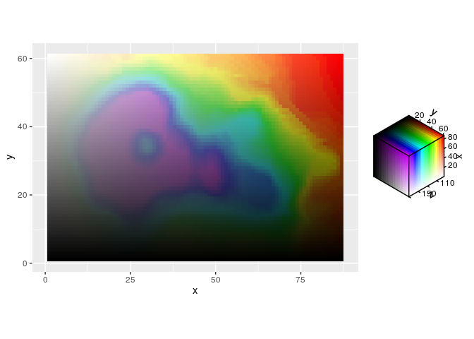
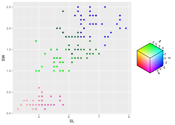
Perhaps a use-case for chromatic scales is when the interpretation of a variable isn’t directly related to a property of the data points. For example, embeddings project data into a new space which might preserve some properties, such as distance between data points, but wherein dimensions of the new space are meaningless on their own. You can use a chromatic scale to map the embedding to colours, which can give a neat ‘flavour’ to the data points through colour.
if (requireNamespace("umap")) {
  set.seed(42)

  # Project the iris dataset into 3D UMAP space
  config <- umap::umap.defaults
  config$n_components <- 3
  umap_3d <- umap::umap(iris[, 1:4], config)$layout

  df <- data.frame(
    SL = iris$Sepal.Length,
    SW = iris$Petal.Width,
    x = umap_3d[, 1],
    y = umap_3d[, 2],
    z = umap_3d[, 3]
  )

  ggplot(df, aes(SL, SW)) +
    geom_point(aes(colour = rgb_spec(x, y, z)))
}
#> Loading required namespace: umap