Coverage

Calculates how often a space is covered by a set of ranges.

stat_coverage(
  mapping = NULL,
  data = NULL,
  geom = "area",
  position = "identity",
  ...,
  trim = FALSE,
  na.rm = FALSE,
  orientation = NA,
  show.legend = NA,
  inherit.aes = TRUE
)

Arguments

mapping	Set of aesthetic mappings created by aes() or aes_(). If specified and inherit.aes = TRUE (the default), it is combined with the default mapping at the top level of the plot. You must supply mapping if there is no plot mapping.
data	The data to be displayed in this layer. There are three options: If NULL, the default, the data is inherited from the plot data as specified in the call to ggplot(). A data.frame, or other object, will override the plot data. All objects will be fortified to produce a data frame. See fortify() for which variables will be created. A function will be called with a single argument, the plot data. The return value must be a data.frame, and will be used as the layer data. A function can be created from a formula (e.g. ~ head(.x, 10)).
geom	Use to override the default connection between geom_density() and stat_density().
position	Position adjustment, either as a string, or the result of a call to a position adjustment function.
...	Other arguments passed on to layer(). These are often aesthetics, used to set an aesthetic to a fixed value, like colour = "red" or size = 3. They may also be parameters to the paired geom/stat.
trim	If FALSE, the default, each density is computed on the full range of the data. If TRUE, each density is computed over the range of that group: this typically means the estimated x values will not line-up, and hence you won't be able to stack density values. This parameter only matters if you are displaying multiple densities in one plot or if you are manually adjusting the scale limits.
na.rm	If FALSE, the default, missing values are removed with a warning. If TRUE, missing values are silently removed.
orientation	The orientation of the layer. The default (NA) automatically determines the orientation from the aesthetics mapping. In the rare event that this fails, it can be given explicitly by setting orientation to either "x" or "y". See the Orientation section of geom_density().
show.legend	logical. Should this layer be included in the legends? NA, the default, includes if any aesthetics are mapped. FALSE never includes, and TRUE always includes. It can also be a named logical vector to finely select the aesthetics to display.
inherit.aes	If FALSE, overrides the default aesthetics, rather than combining with them. This is most useful for helper functions that define both data and aesthetics and shouldn't inherit behaviour from the default plot specification, e.g. borders().

Details

For IRanges and GRanges classes, makes use of the coverage function. When data is numeric, be sure to also set the xend or yend aesthetic.

Note

The Ranges classes as x|y are considered closed-interval, whereas x|y and xend|yend with numeric data are considered open interval.

Aesthetics

stat_coverage understands the following aesthetics (required aesthetics are in bold, optional in italic).

• x

• y

• xend (if data is numeric)

• yend (if data is numeric)

• alpha

• colour

• fill

• group

• linetype

• size

• weight

Computed variables

coverage

coverage

scaled

coverage scaled to a maximum of 1

density

coverage integrated to 1

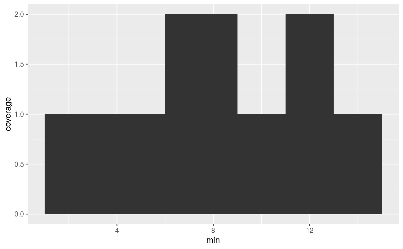
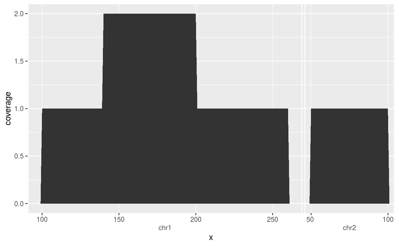
Examples

# Computing coverage on numeric data
df <- data.frame(min = c(1, 6, 11),
                 max = c(9, 13, 15))
ggplot(df, aes(x = min, xend = max)) +
  stat_coverage()

# Computing coverage on Ranges data
require(GenomicRanges)

df <- DataFrame(x = GRanges(c("chr1:100-200", "chr1:140-260",
                              "chr2:50-100")))
ggplot(df, aes(x)) +
  stat_coverage()